One of the most common complaints during a football match is the wrong decision of the referees regarding the offside. This is a very complex rule to impose in real-time, because it depends of the position of the ball and, at least, two players. I find it amazing that the referees are right most of the time without any extra help.
Can we create a model to make a decision based on the position of the players without explicitly setting the rules?
Understanding the problem
A player is in an “offside position” if they are in the opposing team’s half of the field and also “nearer to the opponents’ goal line than both the ball and the second-last opponent.” This is a brief description, and we can develop it a little further by stating the five conditions that must be met.
- A teammate touches the ball, either by a pass, a headbutt or kicking towards the goal;
- The pass is not from a corner kick, a goal kick or a throw-in;
- The receiving player is in the offensive half of the field;
- The receiving player is closer to the goal line than the ball;
- There is only one player from the other team between the receiving player and the goal line.
When all five conditions happen in a given play, the game must be stopped and a free kick is given to the defensive team.
Our goal here is to create a model where these rules are not explicitly written, but are learned from a data set of annotated plays. That is, we are going to feed the model with a series of plays, with the position of the 22 players, 11 for each team, the player who is passing the ball and the receiver, with a label “offside” or “no_offside”. We will evaluate the model afterwards to see how good is the fit.
Available Data
We found some collections of data with offsides, but they didn’t include the position of the players. Furthermore, we also needed data for the cases where no offside happened. There were two possible paths:
- create a large number of plays by choosing randomly the position for all the players;
- find real data from, at least, one football match.
If we go for the first option, it is very easy to generate a large number of plays, but most of them will be unrealistic for a football match. In other words, easy, but too much junk.
If we go for the second option, we are sure to have real situations from a football match, but it is very hard to find such data. If found, data cleaning will be necessary, and need for data augmentation will be strong.
Jackpot: we found ONE match!
We have found a data set called Magglingen2013.
Recorded position data of professional football matches. The data includes positions on football field in 100ms steps (10Hz) of the players, and the ball.
The games were performed in real competition situation by top swiss football club players (U19). The data was intentionally anonymized, not at last because of the high density of information available.
This dataset gives you a glimpse on a possible data stream originating from a live match in some not to distant future.
The terrain was an artificial green. Recordings are available from beginning of the first half time up to the end to the second half time.
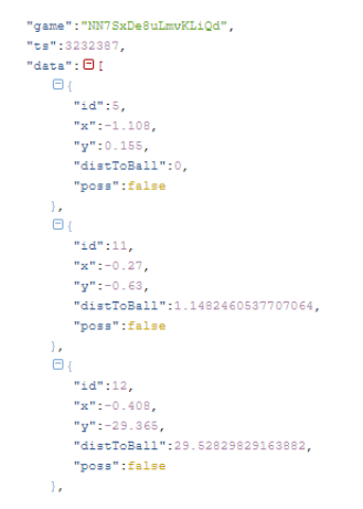
There are two matches listed at this website, but the links are broken. We were able to find the file for “Game TR vs. FT“, so we are using that as our initial data set. The file is a JSON file, with a timestamp and, for each player, an identifier, the coordinates on the field (x,y), the distance to the ball and if he has the possession of the ball.
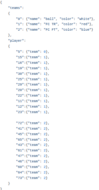
There is a second JSON file, matching the player ID with one of the two teams, and another ID for the ball itself.
Data Exploration and Data Cleaning
We need to understand the data to be able to clean it and create our models. For example, the size of the field is a very important measure!
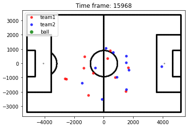
We start by creating a table where each row is one instant of our match (68.031 in total) and the columns are the positions x and y for the players, in the order show in the above figure. We won’t be using the ball’s position, because we will generate lots of new plays by varying who is passing the ball and who is receiving it.
The first step is to replace the value 99999 with NaN. There are missing data for some of the timestamps, where the position of one or more players were not recorded, and also for the half time break.
Let’s take a look at the distribution for the x and y for all players. With these histograms, we will be able to estimate the length and the width of the field.
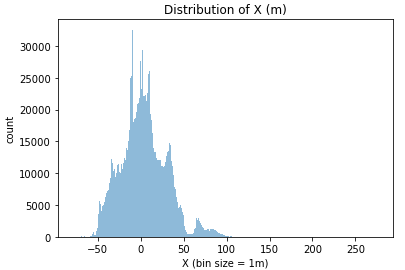
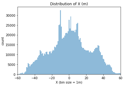
From these histograms, we learn two things:
- The X position is in the direction of the length of the field, with the center at 0 and the goal lines at +/- 52m;
- We need to clean more data, getting rid of all the positions where the players are more than 2 meters off the field (to allow corner kicks and the goalies retrieving the ball).
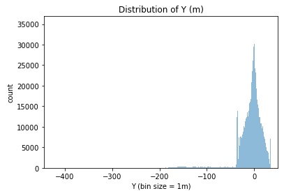
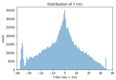
From these histogram, we learn two things:
- The Y position is in the direction of the width of the field, with the center at 0 and the side lines at +/- 34m;
- We need to clean more data, getting rid of all the positions where the players are more than 2 meters off the field (to allow the throw-ins).
The next step in cleaning the data is to replace all the X positions outside the range [-52,52] and all the Y positions outside [-34,34] with NaN, because they must be some malfunction of the sensors.
We have now a new problem. From the original 68.031 rows, we have a varying number of valid values for each column (position of each player). The lower count is for player #16, with 41.801 valid positions, which means he probably was sent off or got hurt in the beginning of the second half.
We have two options:
- Fill in the gaps in the data, with an average position or a new random location;
- Remove all the rows with missing data.
Our data has a frequency of 10Hz, that is, a sequence of 10 rows is equivalent to 1 second. We won’t miss out on anything special if we remove just one row. Let’s see what are the largest sequences of rows with missing data.
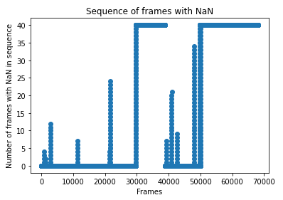
In the first half, there is an event with 4 rows in a sequence with at least one NaN, another sequence with 12 rows, another with 7 rows, and one with 24 rows. Then we see the end of the first half and the return of the game. We see four sequences (with 6, 20, 8 and 35 rows). After these events, we see what was expected: one player is out for the remainder of the game.
We have three different groups:
- Half-time
- One player out
- Problematic data
It is important here to remember that the data has a frequency of 10Hz. A sequence of 35 rows, our largest sequence, is equivalent to 3.5 seconds of the game.
To keep things simple, we can get rid of all the time frames with incomplete data without compromising our analysis.
Before we do that, let’s make a transformation that will simplify our work later on. The teams trade sides for the second half. We will flip the data for the second half, multiplying the positions by -1, so that the team’s offensive half is always the same, team 1 attacking to the right and team 2 to the left.
From the original 68031 frames, we have 27505 incomplete rows. This leaves information for 40526 frames, equivalent to 67 minutes and 32 seconds, about 75% of a match. Good enough for us!
Data Augmentation
We have more than 40 thousand situations, but let’s pump up those numbers! We will create new data by adding noise to the positions of the players. By doing this, we are getting new plays, keeping them similar to real ones. For each row in our data set, we will add two new rows, with a small random change in the position of every player.
We now have more than 120k plays in our data set. For finish the input for our models, we need to include three new columns: the passing player, the receiving player and the flag “offside/no_offside”. There are 22×22 = 484 possibilities, including the ball coming from the other team and the player keeping the ball. With our 121.578 plays, we could have a total of 58.843.752 different game situations. This might be a problem, so we are going to randomly select 25 possibilities instead of the 484, leaving us with close to 3 million game situations. For simplicity, the passing and receiving player will be defined by the order of the lineup, that is, these columns will be filled by numbers between 1 and 22.
From our original 68.031 timestamps, we end up with 3.039.450 different plays. We are ready to annotate the data set, that is, determine for each row if the play is valid or an offside should be called.
Data Annotation and Creation of a Balanced Input Data set
A player is in an “offside position” if they are in the opposing team’s half of the field and also “nearer to the opponents’ goal line than both the ball and the second-last opponent.” This is a brief description, and we can develop it a little further by stating the five conditions that must be met.
- A teammate touches the ball, either by a pass, a headbutt or kicking towards the goal;
- The pass is not from a corner kick, a goal kick or a throw-in;
- The receiving player is in the offensive half of the field;
- The receiving player is closer to the goal line than the ball;
- There is only one player from the other team between the receiving player and the goal line.
When all five conditions happen in a given play, the game must be stopped and a free kick is given to the defensive team. We need to include two new conditions:
- The receiving player is not the same as the passing one. This means the player can keep the ball to himself even if the above conditions happen.
- The receiving player must be in the field. The passing player can be outside, when we consider the play a throw-in or a corner kick.
For each game situation previously created, we will evaluate these 7 conditions. The offsides will be a small subset of the total plays. Besides checking for offsides, we are creating a number of groups to help creating a more balanced dataset:
- when all 7 conditions are met, the offsides;
- when just one of the other conditions is not met, the “close call” non offsides, but excluding condition 5;
- when the only condition avoiding an offside is the number of players between the receiving player and the goal line, condition 5, because this is expected to be the most recurring one;
- when all 7 conditions aren’t met;
- all the other non offside cases.
This is the most time consuming step in the analysis.
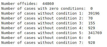
We want to create a balanced input data set, with half of them offsides. We start by selecting the harder cases, when just one of the conditions isn’t met, excluding rule #5. With that, we have 41.278 plays. We pick the same number of cases from the cases with rule #5, and end up with 82.556.
We mapped 427.837 plays in the figure above. That means there are more than 2.5 million other situations. We will pick the same number as above, getting our set to 165.112, all plays where there is no offside. We need the same number of offsides, so there will be another data augmentation step.
Second Data Augmentation
We have 44.860 offside plays and we need to get this number up to 165.112 to balance our data set. We need to increase the number of plays with offsides. The solution is quite simple: excluding throw-ins and corner kicks, the conditions are independent of Y. We will generate new plays by altering the position y for the players not involved in the play.
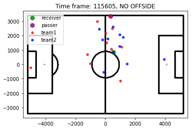
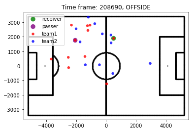
After this step, we have our final data set, with 330.224 plays, half in each class offside/no-offside! Before moving on, let’s plot some random examples to see if everything is right.
Classification models
Two different classification models will be evaluated: Random Forest and Support Vector Classifier. For the RF model, we will vary the number of decision trees (1, 10, 100, 1.000 and 10.000). For the SVC model, much more computation-intensive, we will vary the size of the training set (25%, 50% and 75%). At the end, we will compare their performances using ROC, Accuracy and Confusion Matrix.
Random Forest Classifier
Five different Random Forest models will be generated, with 1, 10, 100, 1.000 and 10.000 trees. We are using 75% of the data as a training set. Below, we have tables showing the metrics for each model.
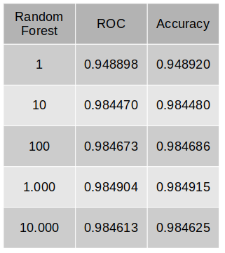
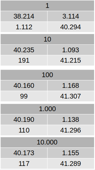
According to our metrics, the best model is the Random Forest with 1.000 trees, with an accuracy of 98.49%! Even our simplest model, with just one tree, has an accuracy of 95%.
Support Vector Classifier
This method has a higher computational cost, so we are running three different models, with 25%, 50% and 75% of the data as a training set. Below, we have tables showing the metrics for each model. To be able to compare the confusion matrices, as we have test sets with different sizes, we also show the results in percentage.
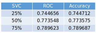
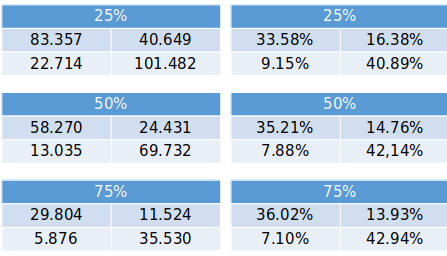
According to our metrics, the best model is the Support Vector Classifier with 75% training set, with an accuracy of 78.97%, way lower than our Random Forest models.
Evaluation of the models
To our surprise, the Random Forest Classifier, with 1.000 trees, was the best model! We were expecting the SVC to be a better fit, because the offside conditions use the relative position of the players and a higher dimensional method would be able to get a better understanding of the data.
When we compare the best RF to the best SVC, our RF performance is way better, with an error close to 1.5%! Very impressive result with such a simple model.
Final conclusion: we created a model to make a decision based on the position of the players without explicitly setting the rules with an accuracy of 98.5%.
Jupyter Notebook available at Github. Interactive panel at Tableau Public.