The Brazilian Football Championship is the main tournament of the most popular sport in Brazil. Most of the country is represented through one of the twenty teams (the Northern region was present in former editions). Brazil is a continent-sized country, so this tournament involves long trips, specially for teams in the Northeast region.
Starting with a set of conditions that will be discussed later, we will use Genetic Algorithms to propose a possible sequence of matches that minimize the impact of these long trips, although it is very clear there are teams who are geographically distant from the rest and there is no way to have every team with the same total distance. We try three different metrics for this optimization, all of them based on the distances traveled by each team.
This kind of problem is known as TTP, Traveling Tournament Problem. There is a huge number of possible combinations and it is really hard to get the optimum solution, even for a small number of teams.
The 2020 Championship
It is very hard to create from scratch a table with the matches for each round. For this project, we will use the table of matches from the 2020 Championship. We will try to improve on that with our algorithm.
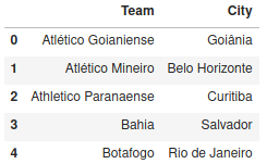
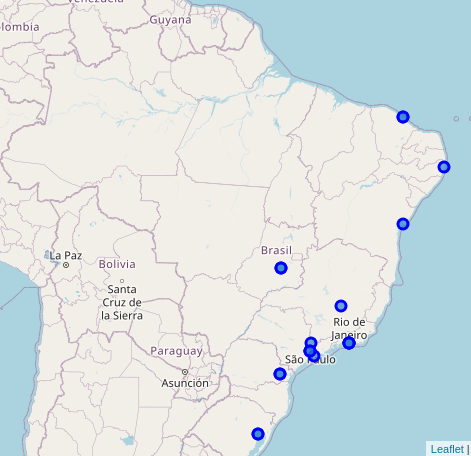
We need the list of the twenty teams with their home city. As we are interested in the distance traveled by each team, we will get the coordinates (latitude and longitude) for the center of the city as an approximation.
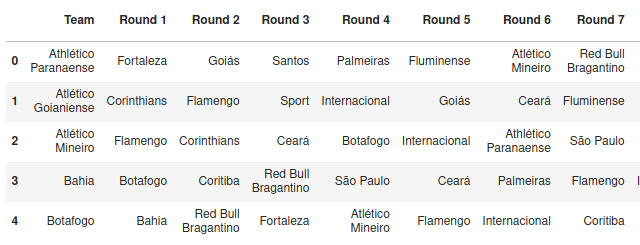
We have the match sequence for each of the twenty teams for the 2020 Championship. There are two halves, where the second one repeats the order of the first, but flipping the home and away teams. Taking this into account, we only need to worry about the first half.
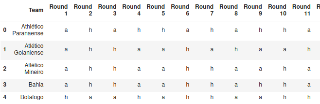
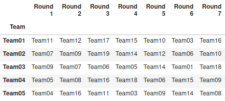
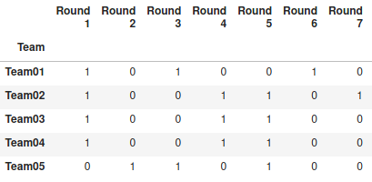
We represent the matches for the first half with two tables, one with the opponents in each round and another telling us if the team plays at their home stadium or away (h or a).
Data Transformation
We need to modify the table so that we can update the list of teams. We will replace each team by their position in the alphabetical order. For example, Athlético Paranaense will be replaced by Team01, Atlético Goianiense by Team02, and so on. We will have three generic tables.
Definition of the problem
This kind of problem is very complex, as there are too many possible combinations. For the Brazilian Championship, it is probable that the full table of matches is made by hand, with only one assumption:
- No team can play more than two rounds in a row at home or away.
For our exercise, we will work with an Express Tournament. The number of rounds is the same, but we add another condition:
- The teams don’t return to their home city, going from one match to the location of the next.
This new condition is only relevant to our evaluation metric. Without this condition, the total distance traveled by each team would be the sum of distance from their home cities to all the others. By adding this artificial condition, we are able to run our algorithm. The other option would be to develop a more complex metric.
We have three tables to work with. To get the optimum results, we should make changes in all of them at the same time, but this is rather difficult. Let’s tackle one at a time, leaving the other two fixed.
For each case, we will create a initial set of possible configurations, represented by a vector or a matrix. They will be our genes for the genetic algorithm. These are evaluated based on the metrics we propose and the best ones will be used to generate a new set of configurations. This process is repeated a pre-determined number of times and should result on an optimized result.
Order of teams – We are going to make changes in the order of the teams, keeping the matches and location tables fixed. That means defining which team is ‘Team01‘, which one is ‘Team02‘, until ‘Team20‘. The original list is in alphabetical order. There are 2432902008176640000 possibilities for this set of teams.
In this case, our gene is a vector with the numbers from 1 to 20. The numbers represent each team in the alphabetical order, and the position in the vector represents the position in the generic list. That is, if the first number in the vector is 5, the fifth team in the alphabetical list will be ‘Team01‘. The mutation for each generation is the selection of two positions in the vector and swapping the teams.
Match location – We are going to make changes to the location table, keeping the order and matches tables fixed. That is, define the sequence of home and away matches for each team. It is important to respect the condition that no team can play more than two games in a row at home or away.
In this case, our gene is a 20×19 matrix, where each row is the location of the matches for a team and each column is a round. The mutation is to pick a single match in the matches table and swap the home team. It is a valid mutation if the condition above is met.
Match order – We are going to make changes to the matches table, keeping the order of the teams fixed. That is, define the sequence of matches for each team. When we alter the sequence of the rounds, this also affects the location table. It is important to respect the condition that no team can play more than two games in a row at home or away.
To simplify this case, our gene is a vector with numbers from 1 to 19, The numbers represent each round in the original order, and the position in the vector represents the position in the new order. That is, if the first number in the vector is 5, the fifth round in the original order will be considered the first round. The mutation for each generation is the selection of two positions in the vector and swapping the rounds. Again, it is important to respect the condition that no team can play more than two games in a row at home or away.
Distance between cities
We have 20 teams spreading over 11 cities, in 9 states. From the coordinates of the center of each city, we can create the table with the distances between each team.
We have used geopy to get the coordinates of each city and haversine to calculate the distance between them.
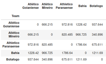
For example, the distance between Bahia and Grêmio is: 2305.24 kilometers.
Evaluation Function
We need to develop a function that gives us a score of a configuration so we can determine the best ones to create the next generation to be tested. This is the function we want to optimize. We will base it on the distance traveled by each team. For example, for ‘Team01‘, the distance between its home city to the location of the first match, plus the distance to the location of the second one, and so on.
We have two conditions in our tournament:
- No team can play more than two rounds in a row at home or away.
- The teams don’t return to their home city, going from one match to the location of the next.
We will try three different metrics, but they all depend on the vector with the total distance traveled by each team.
Our three proposed evaluation functions:
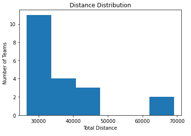
- minimizing the total sum of the distance;
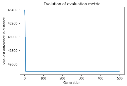
- minimizing the difference between the smallest and the largest distances;
- minimizing the standard deviation of the distribution of distances.
For the original configuration, we have: total distance = 725398.52; difference = 43393.29; standard deviation = 12221.00.
Optimizing the Team Order
We are going to modify the order of the teams while keeping the locations and the matches tables fixed. In other words, we will define what team is ‘Team01, which one is ‘Team02‘, up to ‘Team20‘.
We have four parameters to define:
- the number of genes (configurations) we will evaluate in each generation: 6;
- the number of genes we will use to create the new generation: 2;
- the number of generations: 500;
- the original configurations.
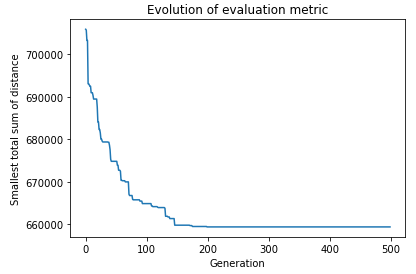
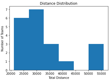
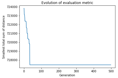
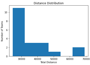
Minimizing the total distance: The best configuration has a total distance of: 659363.85 km, what means we reduced it in 9 %.
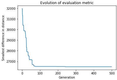
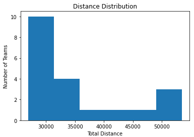
Minimizing the difference between largest and smallest distances traveled: The best configuration has a difference of distance of: 26492.70 km, what means we reduced it in 39 %.
Minimizing the standard deviation: The best configuration has a standard deviation of: 7972.13, what means we reduced it in 35 %.
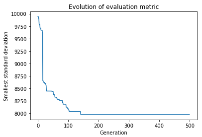
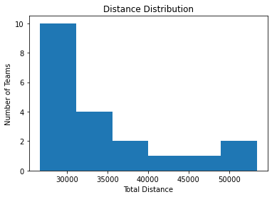
We have finished the optimization using only the order of the teams. Looking at the distances and their distributions, it seems that the third option, the standard deviation, is the most egalitarian one.
Optimizing the Locations table
We are going to modify the location of the matches while keeping the order of the teams and the matches table fixed. In other words, we will define the sequence of home and away games for each team, respecting the condition that no team can play more than two games in a row at home or away.
Minimizing the total distance: The best configuration has a total distance of: 717442.19 km, what means we reduced it in 1 %.
Minimizing the difference between largest and smallest distances traveled: The best configuration has a difference of distance of: 42490.59 km, what means we reduced it in 2 %.
Minimizing the standard deviation: The best configuration has a standard deviation of: 12101.67, what means we reduced it in 1 %.
Our results in this case are much worse than the ones optimizing the order of the teams. When we compare the improvements, we also see lower values.
Optimizing the Match table
We are going to modify the order of the rounds while keeping the order of the teams fixed. In this case, we will need to alter the location table too. In other words, we will modify the order of the columns in the matches table and also in the locations table. We still need to validate the condition that no team can play more than two games in a row at home or away.
We had to stop this run, because it wasn’t able to find new valid configurations. This is independent of the evaluation function, so we won’t be proceeding with this kind of optimization.
Conclusion
The Traveling Tournament Problem is really complex, and creating a competition with 20 teams is very hard. We split the problem in three tables and tried approaching the task one by one. Even so, we were able to move forward with two of them.
We found that changing the order of the teams has a bigger impact than modifying the location of the games. In the former, we had a maximum distance traveled close to 54k kilometers, while in the latter it was close to 70k.
This solution can be applied to any new Brazilian Championship. For the 2021 edition, we should update the list of teams and their cities, and then run the optimization of the order of the teams using the standard deviation as an evaluation metric.
Final Conclusion: we can generate an optimized tournament using genetic algorithms by modifying the order of the teams using standard deviation as an evaluation metric.
Jupyter Notebook available at Github.